Inventory management feels like gambling
Managing inventory usually feels like a gambling addiction. You place a wager on how much product you need, and the market either rewards you or punishes you. Order too much, and your cash gets trapped in a warehouse, gathering dust. Order too little, and you face the nightmare scenario: stockouts and lost revenue.
Most inventory managers treat this as a "gut feeling" exercise. But that's not you.
EOQ removes emotion from purchasing decisions. You are looking for the point where the math stops you from bleeding money. This is where Economic Order Quantity (EOQ) steps in.
EOQ is the calculation that identifies the ideal order size to minimize costs. It removes the emotion from purchasing and replaces it with efficiency. We are going to break down the variables, walk through the formula using real numbers, and then look at how modern AI is rewriting the rules of this decades-old concept.
What is EOQ? A one-paragraph definition
EOQ stands for Economic Order Quantity. It is the order size that minimizes the total annual cost of buying and holding a product — the point where what you spend placing orders and what you spend storing stock add up to the smallest possible number. The EOQ model was first published by Ford W. Harris in 1913 and is still taught as the baseline inventory equation in supply chain management, sometimes under the name the Wilson formula.
The short version of the EOQ equation:
EOQ = √(2DS / H)
Where D is annual demand in units, S is the cost of placing one order, and H is the cost of holding one unit for one year. The rest of this guide unpacks each variable, works a full example, and shows where the model breaks.
The Core Concept: Balancing Two Opposing Costs
EOQ balances ordering costs against holding costs
Inventory management fights a battle between two financial enemies that pull your business in opposite directions: Ordering Costs and Holding Costs.
Ordering costs drop when you buy in bulk. On one side, you have Ordering Costs. These are the expenses you pay every time you contact a supplier. The logic is simple: if you order massive batches, your ordering costs plummet because you pay for shipping and setup less often. Anything that reduces the manual work in your purchase management process reduces this number directly.
Holding costs rise when you buy in bulk. On the other side, you have Holding Costs. These are the silent budget-killers—the costs of storing and insuring stock. The more you order at once, the heavier this burden becomes. Your warehouse fills up. Your insurance premiums rise. Your cash is tied up in physical goods rather than growth-driving initiatives.
EOQ is the point where total inventory cost is lowest
If you graph these two costs, they form an "X." Somewhere in the middle, there is a single point where the combined cost of ordering and holding is at its absolute mathematical minimum.
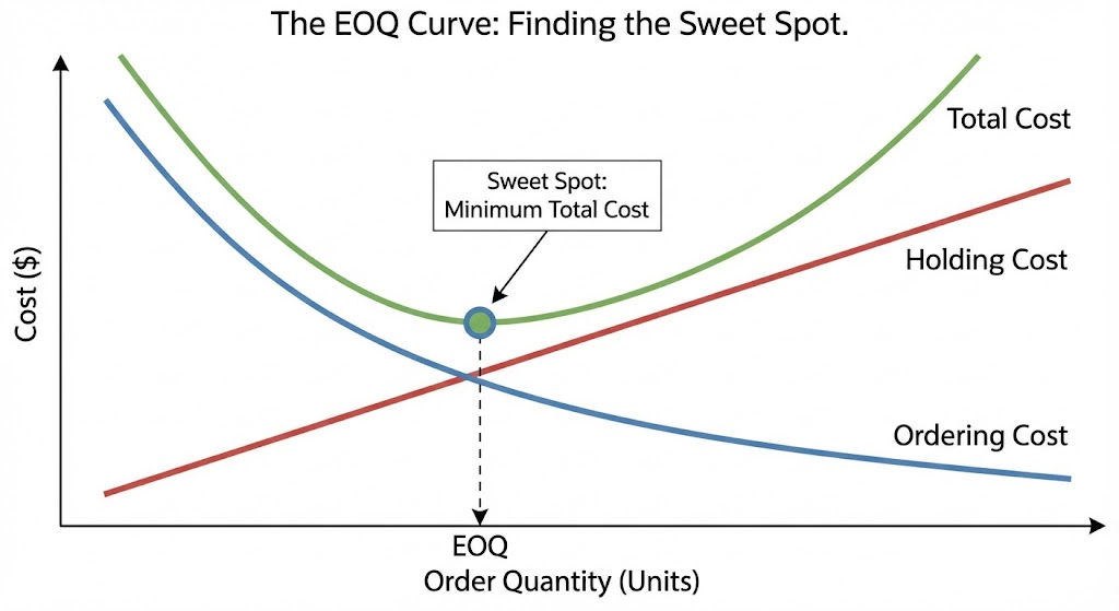
That point is the EOQ. It creates a balance—ensuring you aren't wasting cash on frequent, tiny orders, nor drowning in excess stock.
At the EOQ, ordering cost and holding cost are equal
Here is the property that makes the EOQ graph click. At the exact bottom of the total cost curve, your annual ordering cost and your annual holding cost are the same number. The two lines cross precisely at the optimum.
That gives you a free sanity check. Calculate your EOQ, then calculate both costs separately. If they don't land within a rounding error of each other, you have made an arithmetic mistake somewhere. We will prove this with real numbers further down.
The Three Pillars (Variables) of EOQ
To solve the puzzle, you need three specific pieces of data.
D = Annual demand, the units you'll sell in a year
This is the total number of units you expect to sell over the coming year.
Don't just look at last month and multiply by twelve. You need to look at historical data to get a number that reflects reality. If you operate in a volatile market, this number can be tricky (we'll discuss how AI fixes this later), but for the standard formula, you need a solid annual estimate.
S = Order cost, the flat fee per purchase order
This variable represents the flat fee associated with processing a purchase order.
Crucially, this is not the purchase price of the widget itself. This is the cost of the action of ordering. It includes shipping fees, handling charges, and the hourly wage of the procurement manager creating the PO. Whether you order 1 unit or 1,000 units, this setup cost remains largely the same—which is why high order costs encourage bulk buying.
H = Holding cost, the yearly cost to store one unit
This is the cost to store a single unit for one full year.
Businesses often miscalculate this variable. It includes warehousing rent, utilities, security, and insurance. But the biggest component is opportunity cost (the money sitting on a shelf that isn't growing). A good rule of thumb? Holding cost is usually 20% to 30% of the total inventory value.
The holding cost formula. Most teams don't have a per-unit storage figure sitting in a report, so they derive it:
H = unit cost × carrying cost rate
A smartwatch that costs you $16 landed, carried at a 25% rate, gives you H = $16 × 0.25 = $4 per unit per year. Getting this rate honest is a cost accounting exercise, not a guess — and because H sits in the denominator, understating it inflates every EOQ number you produce.
The Formula and Calculation
Now that we have our variables, we can plug them into the framework. The formula is a simple way to slice through the noise.
The Formula
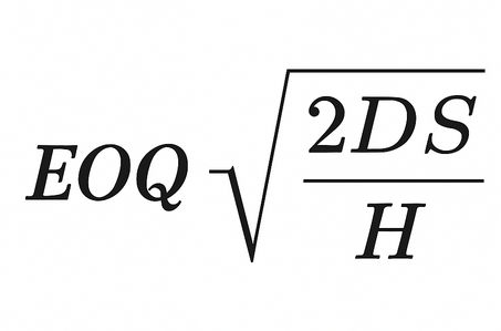
It reads as: The square root of (2 times Annual Demand times Order Cost) divided by Holding Cost.
Written out as an equation: EOQ = √(2DS / H), sometimes shown as Q* = √(2DS/H). You will also see the optimal order quantity formula written with different letters — A for annual usage, O for order cost, C for carrying cost — but the math is identical.
EOQ example: Archer Electronics sells 2,400 smartwatches a year
Let's apply this to a real-world scenario.
Archer's scenario and goal. "Archer Electronics" sells 2,400 smartwatches a year. They want to know exactly how many watches to buy in a single batch to keep costs low.
Archer's three EOQ variables:
- $D$ (Annual Demand) = 2,400 units.
- $S$ (Order Cost) = $50. (This covers the admin time and shipping setup for each order).
- $H$ (Holding Cost) = $4. (It costs $4 to keep one watch on the shelf for a year).
Calculating Archer's EOQ:
- Multiply the numerator:
$2 \times 2,400 \times 50 = 240,000$
- Divide by the denominator (Holding Cost):
$240,000 / 4 = 60,000$
- Take the square root:
$\sqrt{60,000} \approx 245$
Archer should order 245 smartwatches per batch. Archer Electronics should order 245 units at a time.
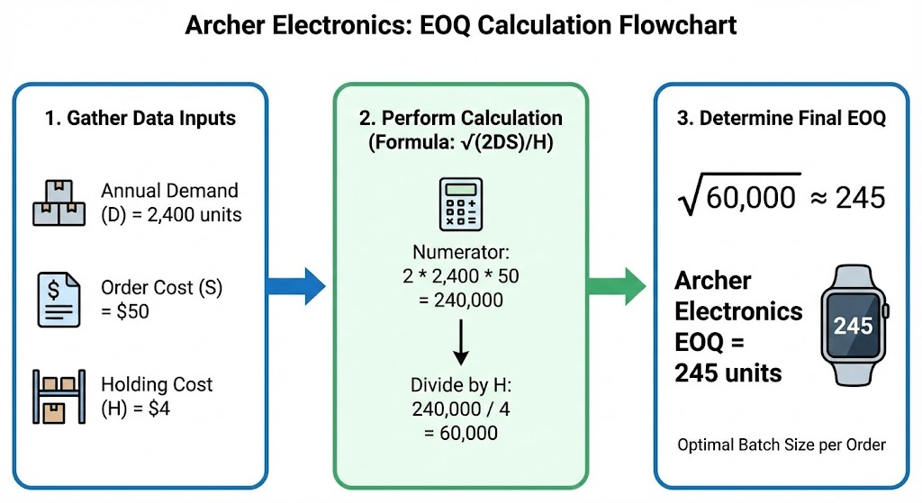
If they order more than 245, their holding costs will eat their profits. If they order fewer, their ordering costs will spike. 245 is the mathematical "sweet spot."
Archer will place roughly 10 orders per year
Once you have the EOQ, you can determine your rhythm. If Archer needs 2,400 units a year and orders 245 at a time, they will place roughly 10 orders per year ($2,400 / 245 = 9.8$). This turns a vague strategy into a concrete schedule.
The number of orders per year formula: $D / EOQ$.
The time between orders formula: $EOQ / D \times 365$. For Archer, $245 / 2,400 \times 365 = 37$ days. Roughly one purchase order every five weeks.
The total annual cost formula: proving 245 is optimal
The EOQ equation tells you how much to order. The total cost formula tells you what that decision actually costs — and lets you prove no other order size beats it.
Total annual inventory cost = (D / Q) × S + (Q / 2) × H
The first term is your annual ordering cost. The second is your annual holding cost, based on average inventory being half your order size. Run Archer's numbers at three different order quantities:
Three things fall out of this table. The EOQ row is the cheapest. Ordering cost and holding cost are identical at the EOQ — $490 each — exactly as the curve predicted. And the penalty for guessing is real money: ordering 500 at a time costs Archer an extra $260 a year on a single SKU. Multiply that across a catalog of a few thousand SKUs and the number stops being academic.
EOQ tells you how much to order, not when
This is the single most common misreading of the model. EOQ answers one question: what is the optimal order size? It says nothing about timing.
The companion calculation is the reorder point, and it uses a different formula:
Reorder point = (average daily demand × lead time in days) + safety stock
Archer sells about 6.6 units a day ($2,400 / 365$). If their supplier needs 10 days to deliver, they hit the reorder point at 66 units, plus whatever safety stock they hold to absorb variability. So the complete policy reads: when stock drops to roughly 66 units, order 245 more.
You need both numbers. EOQ without a reorder point means you know the right batch size and still run out. A reorder point without EOQ means you always order at the right moment and always order the wrong amount.
EOQ vs. MOQ: two different numbers
EOQ is what your math says is optimal. MOQ (minimum order quantity) is what your supplier will accept. They frequently disagree.
If Archer's supplier enforces a 500-unit MOQ, the EOQ of 245 becomes a reference point rather than an instruction. The useful move is to calculate the cost gap — here, $260 a year — and use it in the negotiation, or to compare that penalty against the cost of qualifying a second supplier.
Critical Limitations: When EOQ Fails
EOQ assumes a frictionless supply chain that doesn't exist
The standard EOQ formula assumes you live in a reality where customers buy products evenly and suppliers deliver instantly. Real supply chains are messy. They are full of friction and human error.
Three EOQ assumptions that break in the real world
- EOQ ignores seasonal demand. The formula assumes constant demand. If you sell swimsuits, your "annual demand" is useless in December. Using a flat EOQ here leaves you overstocked in winter and stocked out in summer.
- EOQ ignores supplier lead times. It assumes stock arrives the moment you order it. If you hit your reorder point and the boat gets stuck, the math won't save you.
- EOQ ignores price changes. It assumes purchase price doesn't change. If a supplier raises prices next month, your previous EOQ calculation is instantly obsolete.
Using EOQ blindly in a volatile market causes trouble—but understanding these limitations allows you to use the number as a baseline.
Where EOQ is still worth running
The limitations argue for narrowing the model's scope, not abandoning it. EOQ earns its keep on stable, predictable, high-volume items — the A-class SKUs in an ABC analysis, where consistent demand makes the assumptions roughly true and the dollar savings are large enough to matter.
It earns much less on slow-moving C-class items, on anything seasonal, and on products with volatile input costs. Deciding which SKUs deserve the calculation is itself part of a working inventory management process.
Modern Alternatives and Adjustments
Supply chain management has evolved from pen-and-paper math to predictive intelligence. Here is how modern businesses upgrade the old formula.
Quantity discounts can override the EOQ number
Sometimes, the math says "order 245 units," but the supplier says, "If you order 500, I'll drop the price by 10%."
In this case, the lower purchase price might outweigh the higher holding cost. You need to run a Quantity Discount Model calculation to see if the savings justify the heavier inventory load. High-volume discounts often subsidize the cost of extra warehousing.
The comparison is straightforward once you have the total cost formula above: add the annual purchase cost ($D \times$ unit price) to each scenario's total, then pick the smaller number. The discount wins only when the price saving exceeds the extra holding cost it creates.
Just-in-time inventory eliminates storage instead of optimizing it
This methodology rejects the idea of "holding" inventory entirely. Instead of optimizing batch sizes, JIT aims to reduce Setup Costs ($S$) and Holding Costs ($H$) to near zero.
The goal here is flow—materials arrive exactly when production needs them. In a JIT environment, the EOQ formula is irrelevant because the goal is not to balance costs, but to eliminate storage.
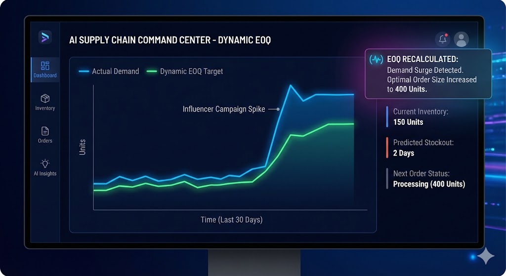
Dynamic EOQ recalculates demand in real time
Modern ERP systems don't just use a static "D" for demand. They use machine learning to create a Dynamic EOQ.
What AI-driven ERPs track to adjust EOQ weekly. These systems analyze real-time trends, weather patterns, and marketing campaigns to adjust the "Demand" variable week-to-week.
Instead of a single EOQ number for the year, you get a number that breathes with the market. If an influencer mentions your product and demand spikes, the system recalculates the optimal order size instantly—ensuring you capture the revenue without blowing up your storage costs.
This is the practical difference between a spreadsheet and AI inventory management: the spreadsheet gives you one number in January, and the system gives you a current one every week. It is also what makes predictive replenishment possible — order quantity and order timing recalculated together, against live demand rather than last year's average.
Conclusion
EOQ is a baseline, not an inventory law
EOQ gives you a starting point for efficiency. It cannot survive the friction of the real world on its own.
How to use EOQ alongside modern inventory software
Start with the formula to understand your financial baseline. But as you scale, you will need to layer in modern software to adjust for lead times and seasonality. Your inventory strategy—for you—is a living system. Keep measuring. Keep optimizing.
If you want the EOQ calculation running against live demand instead of a static annual estimate, see how Tailor handles it.
Frequently Asked Questions
What does EOQ stand for?
EOQ stands for Economic Order Quantity. It is the order size that produces the lowest total annual cost of ordering and holding a given product.
What is the EOQ formula?
EOQ = √(2DS / H), where D is annual demand in units, S is the cost of placing one order, and H is the cost of holding one unit for one year. Multiply 2 by annual demand by order cost, divide by holding cost, then take the square root.
How do you calculate EOQ step by step?
Four steps. First, establish annual demand (D) from historical sales. Second, calculate your cost per purchase order (S) — admin time, shipping setup, handling, but not the price of the goods. Third, calculate holding cost per unit per year (H), usually unit cost × a carrying rate of 20–30%. Fourth, apply √(2DS / H). Confirm the result by checking that annual ordering cost and annual holding cost come out equal.
What are the assumptions of the EOQ model?
The model assumes demand is constant and known, lead times are fixed and reliable, the purchase price per unit doesn't change, ordering and holding costs stay stable, and stockouts never occur. Every one of those assumptions is an approximation in a real supply chain, which is why EOQ is a baseline rather than a policy.
What is the difference between EOQ and reorder point?
EOQ determines how much to order. The reorder point determines when to order, calculated as (average daily demand × lead time) + safety stock. You need both to run a complete replenishment policy.
Is EOQ still used in supply chain management?
Yes, most often as a sanity check on order sizes for stable, high-volume SKUs, and as the logic underneath the replenishment suggestions in modern inventory management systems. What has changed is that the demand input is now recalculated continuously rather than set once a year.